Riemannian optimization

Open this page in an interactive mode via Google Colaboratory.

Riemannian optimization is a framework for solving optimization problems with a constraint that the solution belongs to a manifold.

Let us consider the following problem. Given some TT tensor \(A\) with large tt-ranks we would like to find a tensor \(X\) (with small prescribed tt-ranks \(r\)) which is closest to \(A\) (in the sense of Frobenius norm). Mathematically it can be written as follows:

\begin{equation*} \begin{aligned} & \underset{X}{\text{minimize}} & & \frac{1}{2}\|X - A\|_F^2 \\ & \text{subject to} & & \text{tt_rank}(X) = r \end{aligned} \end{equation*}

It is known that the set of TT tensors with elementwise fixed TT ranks forms a manifold. Thus we can solve this problem using the so called Riemannian gradient descent. Given some functional \(F\) on a manifold \(\mathcal{M}\) it is defined as

\[\hat{x}_{k+1} = x_{k} - \alpha P_{T_{x_k}\mathcal{M}} \nabla F(x_k),\]

\[ \begin{align}\begin{aligned}x_{k+1} = \mathcal{R}(\hat{x}_{k+1})\\with :math:`P_{T_{x_k}} \mathcal{M}` being the projection onto the tangent space of :math:`\mathcal{M}` at the point :math:`x_k` and :math:`\mathcal{R}` being a retraction - an operation which projects points to the manifold, and :math:`\alpha` is the learning rate.\end{aligned}\end{align} \]

We can implement this in t3f using the t3f.riemannian module. As a retraction it is convenient to use the rounding method (t3f.round).

# Import TF 2.
%tensorflow_version 2.x
import tensorflow as tf
import numpy as np
import matplotlib.pyplot as plt

# Fix seed so that the results are reproducable.
tf.random.set_seed(0)
np.random.seed(0)

try:
    import t3f
except ImportError:
    # Install T3F if it's not already installed.
    !git clone https://github.com/Bihaqo/t3f.git
    !cd t3f; pip install .
    import t3f

TensorFlow 2.x selected.

# Initialize A randomly, with large tt-ranks
shape = 10 * [2]
init_A = t3f.random_tensor(shape, tt_rank=16)
A = t3f.get_variable('A', initializer=init_A, trainable=False)

# Create an X variable.
init_X = t3f.random_tensor(shape, tt_rank=2)
X = t3f.get_variable('X', initializer=init_X)

def step():
  # Compute the gradient of the functional. Note that it is simply X - A.
  gradF = X - A

  # Let us compute the projection of the gradient onto the tangent space at X.
  riemannian_grad = t3f.riemannian.project(gradF, X)

  # Compute the update by subtracting the Riemannian gradient
  # and retracting back to the manifold
  alpha = 1.0
  t3f.assign(X, t3f.round(X - alpha * riemannian_grad, max_tt_rank=2))

  # Let us also compute the value of the functional
  # to see if it is decreasing.
  return 0.5 * t3f.frobenius_norm_squared(X - A)

log = []
for i in range(100):
    F = step()
    if i % 10 == 0:
        print(F)
    log.append(F.numpy())

tf.Tensor(749.22894, shape=(), dtype=float32)
tf.Tensor(569.4678, shape=(), dtype=float32)
tf.Tensor(502.00604, shape=(), dtype=float32)
tf.Tensor(490.0112, shape=(), dtype=float32)
tf.Tensor(489.01282, shape=(), dtype=float32)
tf.Tensor(488.71234, shape=(), dtype=float32)
tf.Tensor(488.56543, shape=(), dtype=float32)
tf.Tensor(488.47928, shape=(), dtype=float32)
tf.Tensor(488.4239, shape=(), dtype=float32)
tf.Tensor(488.38593, shape=(), dtype=float32)

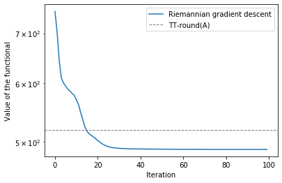
It is intructive to compare the obtained result with the quasioptimum delivered by the TT-round procedure.

quasi_sol = t3f.round(A, max_tt_rank=2)

val = 0.5 * t3f.frobenius_norm_squared(quasi_sol - A)
print(val)

tf.Tensor(518.3871, shape=(), dtype=float32)

We see that the value is slightly bigger than the exact minimum, but TT-round is faster and cheaper to compute, so it is often used in practice.

plt.semilogy(log, label='Riemannian gradient descent')
plt.axhline(y=val.numpy(), lw=1, ls='--', color='gray', label='TT-round(A)')
plt.xlabel('Iteration')
plt.ylabel('Value of the functional')
plt.legend()

<matplotlib.legend.Legend at 0x7f4102dbab70>